home..

Google trend data crawling & visualize

March 2024 (2166 Words, 13 Minutes)

Sole Movie- Google 검색 트렌드 데이터 수집 코드

Google 트렌드에서 “미키17”라는 키워드의 검색량 데이터를 수집하는 코드이다. 현재 날짜는 3월 1일이니, 1월 1일부터 3월 1일 두달 간의 검색량을 얻고 싶었다.

from pytrends.request import TrendReq
import requests
import plotly.express as px

session=requests.Session()
session.get('https://trends.google.com')
cookies_map=session.cookies.get_dict()
nid_cookie=cookies_map['NID']

pytrends=TrendReq(hl='en-US', tz=360, retries=3, requests_args={'headers':{'Cookie':f'NID={nid_cookie}'}})

import pandas as pd
from pytrends.request import TrendReq
import datetime
import time

# pytrends 객체 생성
pytrends = TrendReq(hl='ko-KR', tz=540)

# 관심 있는 키워드 설정
keywords = ["미키17"]

# 트렌드 요청 파라미터 설정 (2024년 2월 동안)
pytrends.build_payload(keywords, cat=0, timeframe='2025-01-01 2025-03-01', geo='KR', gprop='')

# 검색량 데이터를 여러 번 요청할 때 429 에러를 방지하기 위해 시간 간격 추가
def get_interest_over_time(pytrends, keywords):
    while True:
        try:
            data = pytrends.interest_over_time()
            return data
        except Exception as e:
            print(f"Error: {e}")
            print("Sleeping for 60 seconds")
            time.sleep(60)

# 관심 있는 키워드의 검색량 데이터 가져오기
data = get_interest_over_time(pytrends, keywords)

# 데이터프레임에서 "isPartial" 열 삭제
data = data.drop(columns=["isPartial"])

# 현재 날짜와 시간을 사용하여 파일 이름 생성
current_time = datetime.datetime.now().strftime("%Y%m%d_%H%M%S")
file_name = f"search_trend_{current_time}.xlsx"

# 엑셀 파일로 저장
data.to_excel(file_name, index=True)

print(f"Excel file '{file_name}' has been created successfully.")

필요한 라이브러리를 import 한다. 이때 pytrends는 Google 트렌드 데이터를 수집하기 위한 비공식 API 래퍼이다.
Google 트렌드 접근을 위한 세션 및 쿠키 설정

   session = requests.Session()
   session.get('https://trends.google.com')
   cookies_map = session.cookies.get_dict()
   nid_cookie = cookies_map['NID']

Google 트렌드 웹사이트에 접근하여 세션 쿠키를 얻는 과정이다 -> requests.Session()으로 새로운 HTTP 세션을 생성하고, session.get(‘https://trends.google.com’)으로 Google 트렌드 웹사이트에 GET 요청을 보낸다.

session.cookies.get_dict()로 응답에서 받은 모든 쿠키를 딕셔너리 형태로 저장한다.
cookies_map[‘NID’]로 ‘NID’ 쿠키 값을 추출한다. 이 쿠키는 Google 서비스 접근에 필요한 인증 정보를 담고 있다.
pytrends 객체 생성: 언어 설정을 한국어로, 시간을 한국 시간으로 설정.

현재는 검색 키워드를 한 개만 설정했는데, 여러 개 설정할 수 도 있다.

pytrends.build_payload(keywords, cat=0, timeframe=’2025-01-01 2025-03-01’, geo=’KR’, gprop=’’)

완성된 검색 파라미터 이다. 빈 문자열은 웹 검색 결과만 포함한다는 것이다.

에러 방지를 위한 함수 정의

def get_interest_over_time(pytrends, keywords):
    while True:
        try:
            data = pytrends.interest_over_time()
            return data
        except Exception as e:
            print(f"Error: {e}")
            print("Sleeping for 60 seconds")
            time.sleep(60)

Google 트렌드 API의 요청 제한(rate limit)에 대응해야 함 –> pytrends.interest_over_time()으로 검색량 데이터를 요청하고, 요청이 성공하면 데이터를 바로 반환한다.
오류가 발생하면(주로 429 Too Many Requests 에러) 오류 메시지를 출력하고 60초 동안 대기한 후 다시 시도한다.
이런식으로 반복적으로 요청하면서 Google의 API 제한을 우회한다.

data = get_interest_over_time(pytrends, keywords)
data = data.drop(columns=["isPartial"])
current_time = datetime.datetime.now().strftime("%Y%m%d_%H%M%S")
file_name = f"search_trend_{current_time}.xlsx"
data.to_excel(file_name, index=True)

앞서 정의한 함수를 호출하여 검색량 데이터를 수집한다.
그 다음 결과 데이터프레임에서 불필요한 열을 제거한다.
수집한 데이터를 엑셀 파일로 저장하는데, 현재 시간을 연월일_시분초 형식의 문자열로 변환한다.

데이터를 엑셀 파일로 저장하면 끝!

최종 결과

크롤링을 통해 얻은 데이터셋을 시각화 해보았다.
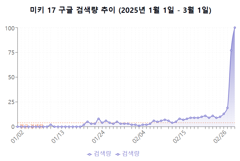
흠…1월 중순부터 검색량이 간헐적으로 나타나기 시작하여 2월 중순까지 소폭 증가하는 추세를 보인다.
데이터는 전형적인 ‘티핑 포인트(tipping point)’ 또는 ‘바이럴 확산’ 패턴을 보여줍니다. 특정 시점(2월 27일경)에 임계점을 넘어서면서 관심도가 기하급수적으로 증가했는데,개봉일이 2월 28일 인 것을 확인하면 그리 놀랄만한 일은 아니다.
홍보가 그리 대대적이지는 않았어서, 아마 개봉 한 달 전에 검색량이 미미했던 것 같다.

n 개의 영화 제목 검색 트렌드 분석 코드

여러 개의 인기영화들의 구글에서의 검색량은 30일동안 어떻게 양상이 나타날까?
넷플릭스에서 한 주동안 인기가 Korea top 이었던 영화들에 대해 검색 패턴을 알아보자.

movie_titles = [
    "싱크홀",
    "외계+인 1부",
    "모가디슈",
    "길복순",
    "기적",
    "장르만 로맨스",
    "발레리나"
]

release_dates = [
    "2021-08-11",  # Sinkhole
    "2022-07-20",  # Alienoid Part 1
    "2021-07-28",  # Escape from Mogadishu
    "2023-03-31",  # Kill Boksoon
    "2021-09-15",  # Miracle: Letters to the President
    "2021-11-17",  # Perhaps Love
    "2023-10-06"   # Ballerina
]
# 영화 제목과 개봉 날짜를 데이터프레임으로 구성
unique_movies = pd.DataFrame({
    "movie_title": movie_titles,
    "week": release_dates
})

# Cweek' 열을 문자열에서 datetime 형식으로 변환하여 각 영화의 개봉일을 기준으로 전후 기간을 계산할 수 있게 함
unique_movies['week'] = pd.to_datetime(unique_movies['week'])

# pytrends 객체 생성
pytrends = TrendReq(hl='ko-KR', tz=540)

# 검색량 데이터를 여러 번 요청할 때 429 에러를 방지하기 위해 시간 간격 추가
def get_interest_over_time(pytrends, keywords, timeframe):
    while True:
        try:
            pytrends.build_payload(keywords, cat=0, timeframe=timeframe, geo='KR', gprop='')
            data = pytrends.interest_over_time()
            return data
        except Exception as e:
            print(f"Error: {e}")
            print("Sleeping for 60 seconds")
            time.sleep(60)

# 결과 저장용 데이터프레임 초기화
result_df = pd.DataFrame()

# 각 영화에 대해 검색량 데이터 가져오기
for index, row in unique_movies.iterrows():
    movie_title = row['movie_title']
    release_date = row['week']
    start_date = release_date - pd.DateOffset(days=15)
    end_date = release_date + pd.DateOffset(days=15)
    timeframe = f'{start_date.strftime("%Y-%m-%d")} {end_date.strftime("%Y-%m-%d")}'
    keywords = [movie_title]

    print(f"Fetching data for {movie_title}...")
    trends_data = get_interest_over_time(pytrends, keywords, timeframe)

    if not trends_data.empty:
        trends_data['movie_title'] = movie_title
        result_df = pd.concat([result_df, trends_data])

# 데이터프레임에서 "isPartial" 열 삭제
if 'isPartial' in result_df.columns:
    result_df = result_df.drop(columns=["isPartial"])

# 현재 날짜와 시간을 사용하여 파일 이름 생성
current_time = datetime.datetime.now().strftime("%Y%m%d_%H%M%S")
file_name = f"search_trend_{current_time}.xlsx"

# 엑셀 파일로 저장
result_df.to_excel(file_name, index=True)

print(f"Excel file '{file_name}' has been created successfully.")

영화 제목과 개봉일을 가져온다.
개봉일 기준 15일 전과 15일 후의 날짜를 계산한다
해당 기간에 대한 검색 트렌드 데이터를 요청.
수집된 데이터에 영화 제목 정보를 추가.
모든 영화의 데이터를 하나의 데이터프레임으로 통합.

시각화 코드

import pandas as pd
import matplotlib.pyplot as plt

# Load the Excel file
file_path = '/content/search_trend_20240712_194816.xlsx'
df = pd.read_excel(file_path, sheet_name='Sheet1')

# Drop rows where all movie search values are NaN
df = df.dropna(how='all', subset=df.columns[2:])

# Set the date column as the index
df.set_index('date', inplace=True)

# Define the new labels for each movie
new_labels = {
    '싱크홀': 'sinkhole',
    '외계+인 1부': 'alienoid part 1',
    '모가디슈': 'escape from mogadishu',
    '길복순': 'kill boksoon',
    '기적': 'miracle: letters to the president',
    '장르만 로맨스': 'perhaps love',
    '발레리나': 'ballerina'
}

# Normalize the date ranges
normalized_df = df.copy()
normalized_df.reset_index(inplace=True)

# Create a new column for the normalized day (1 to 30)
normalized_df['day'] = normalized_df.groupby('movie_title').cumcount() + 1

# Plot the search trends for each movie in the same 30-day period with new labels
plt.figure(figsize=(14, 8))
for original_title, new_title in new_labels.items():
    if original_title in normalized_df.columns:
        plt.plot(normalized_df[normalized_df['movie_title'] == original_title]['day'],
                 normalized_df[normalized_df['movie_title'] == original_title][original_title],
                 label=new_title)

plt.title('Normalized Search Trends for Movies (30-day Period)')
plt.xlabel('Day')
plt.ylabel('Search Volume')
plt.legend()
plt.grid(True)
plt.xticks(rotation=45)
plt.tight_layout()

plt.show()

검색 트렌드 정규화

데이터프레임을 복사하고 인덱스를 리셋. 각 영화별로 그룹화한 후, 날자를 1부터 시작하는 연속된 숫자로 변환.
이렇게 하면 다른 기간에 개봉한 영화들을 동일한 시간축(개봉일 기준)에서 비교할 수 있다.

normalized_df = df.copy()
normalized_df.reset_index(inplace=True)

# Create a new column for the normalized day (1 to 30)
normalized_df['day'] = normalized_df.groupby('movie_title').cumcount() + 1

# Plot the search trends for each movie in the same 30-day period with new labels
plt.figure(figsize=(14, 8))
for original_title, new_title in new_labels.items():
    if original_title in normalized_df.columns:
        plt.plot(normalized_df[normalized_df['movie_title'] == original_title]['day'],
                 normalized_df[normalized_df['movie_title'] == original_title][original_title],
                 label=new_title)

plt.title('Normalized Search Trends for Movies (30-day Period)')
plt.xlabel('Day')
plt.ylabel('Search Volume')
plt.legend()
plt.grid(True)
plt.xticks(rotation=45)
plt.tight_layout()

plt.show()

시각화 : 가로축은 정규화된 날짜,세로축은 Google 검색 볼륨을 나타낸다. 각 영화마다 다른 색상의 선으로 표시되며, 영문 제목으로 범례가 표시된다.

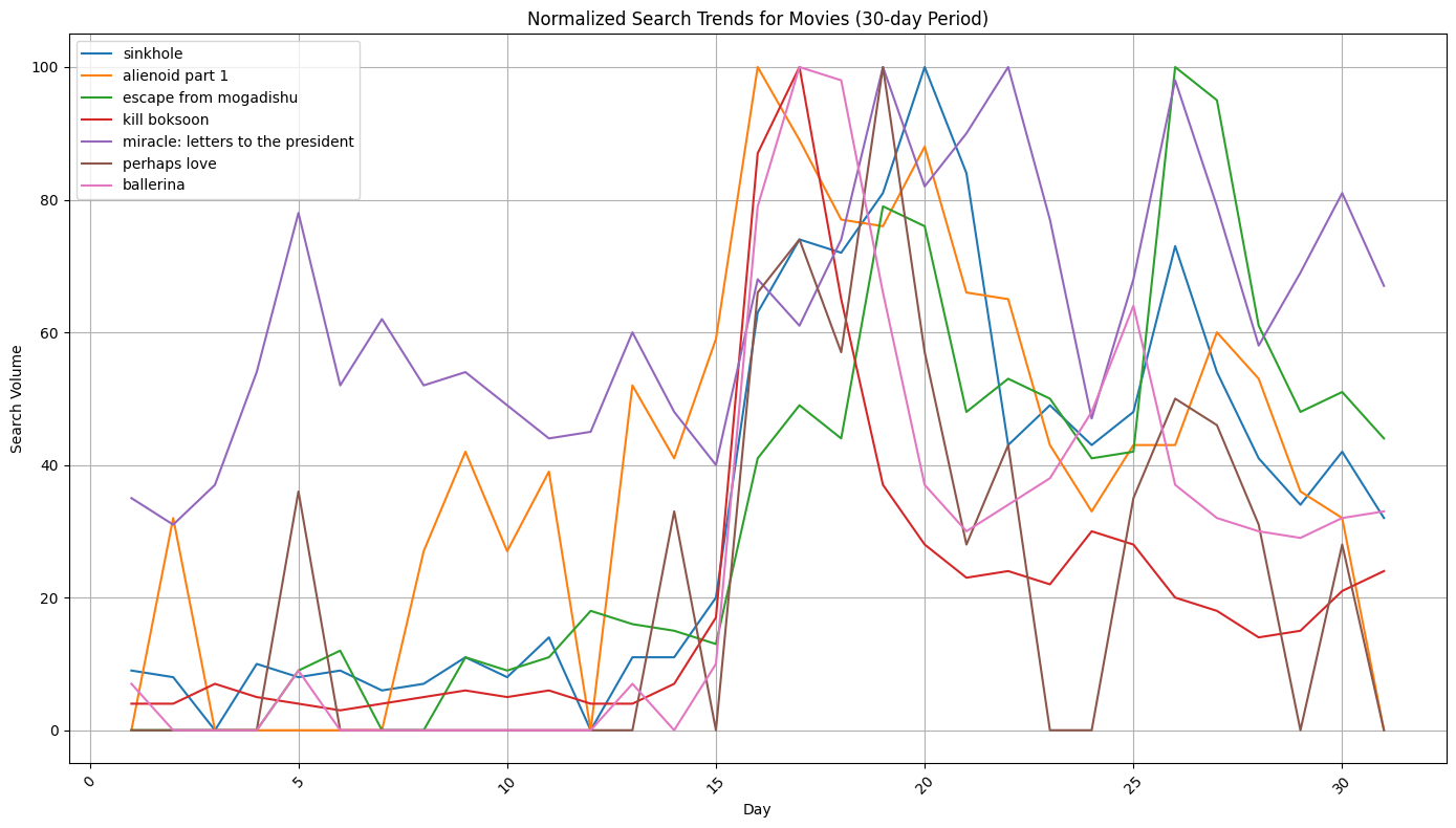
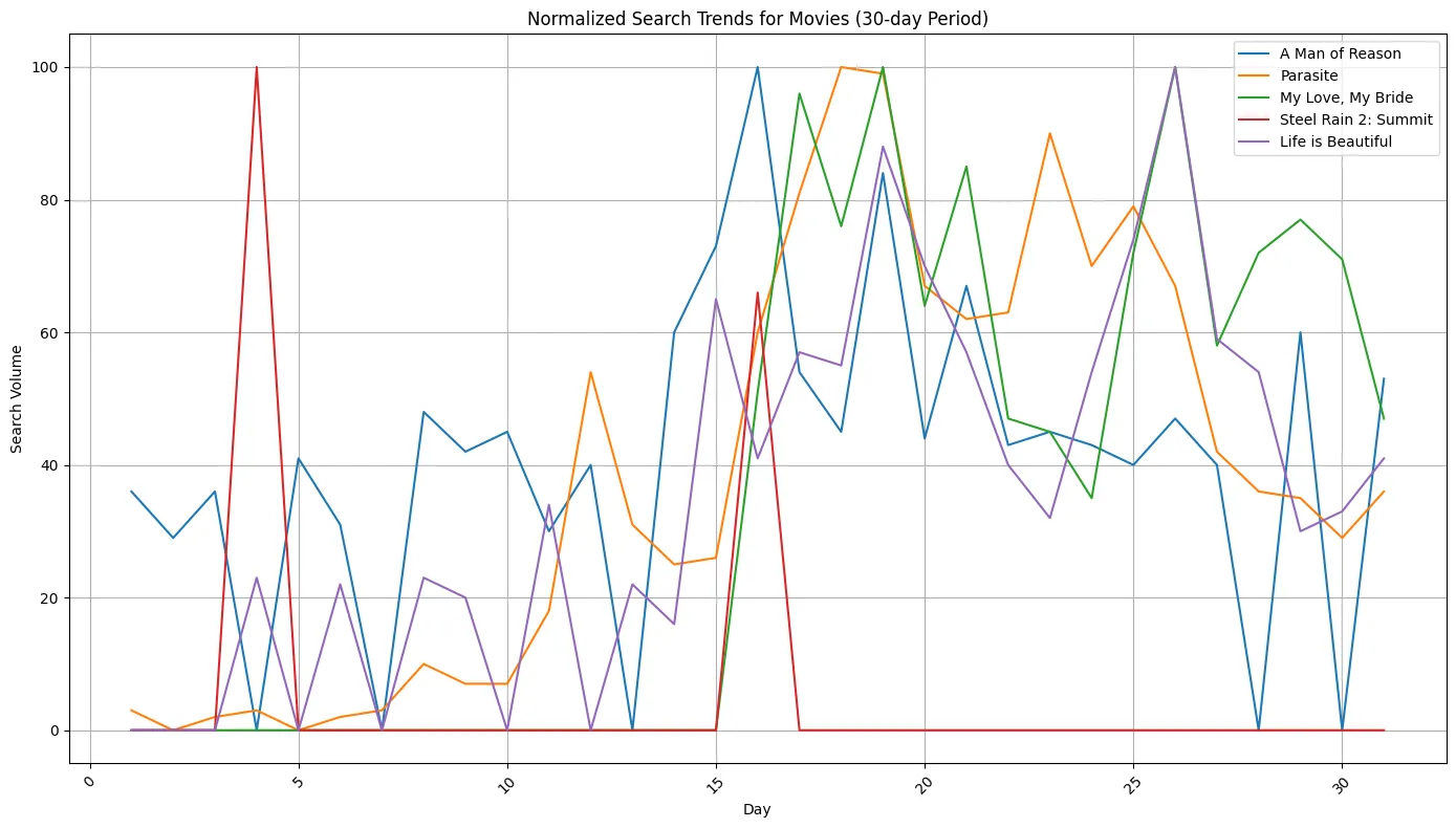
요약: 각 영화가 개봉일(약 15~16일차) 전후로 어떤 검색 트렌드 패턴을 보이는지 분석하고, 서로 다른 7개 영화의 개봉 시점 전후 검색량을 비교하여 어떤 영화가 더 많은 관심을 받았는지 확인할 수 있다. 개봉일에 검색량이 급증하는지, 개봉 전 마케팅 활동으로 인한 검색량 증가가 있는지 등을 파악할 수 있다. (+) 개봉 후 얼마나 오랫동안 검색 관심이 유지되는지를 통해 영화의 입소문 효과나 지속성을 추론할 수 있다!

최종 결과

netflix 첫 주 인기 영화
netflix 첫 주 비인기 영화

개봉일 전후 검색량 패턴

인기 영화(이미지 2): 대부분의 영화가 개봉일(15일차 부근)에 급격한 검색량 상승을 보여준다. 특히 ‘싱크홀’, ‘외계+인 1부’, ‘발레리나’ 등은 개봉일에 거의 최대치(100)에 가까운 검색량을 기록한다.

비인기 영화(이미지 1): 개봉일 전후로 검색량이 더 불규칙하고, ‘스틸레인 2’를 제외하면 개봉일에 명확한 피크가 없다!!!

검색량 지속성

인기 영화: 개봉 후에도 상당 기간(약 20-25일차까지) 비교적 높은 검색량을 유지. 비인기 영화: ‘기생충(Parasite)’을 제외하고는 검색량이 빠르게 감소하거나 더 변동이 심하다.

(+) 이때 기생충은 ‘넷플릭스’ 안에서 순위인 것을 잊지 말도록…!OTT 순위 반영 시 비인기 영화 그룹에 속하지만 인기 영화와 유사한 패턴을 보인 이유가 위 그래프가 기생충이 개봉한 시점에 대한 검색량이니까. 넷플릭스 안에서 비인기인 이유는 , 그저 이미 모든 한국인이 시청을 n 번씩 영화관에서 했을 것이기 때문이다